Ising Anyons and Majorana Fermions

By Iosifina Angelidi, August 2020

In chapter 4.3 of the book, the non-abelian anyonic model of “Ising anyons” is described together with its properties. It is also mentioned that “Ising anyons describe the statistical properties of Majorana fermions”. Below we will prove and explain the correlation of Majorana fermions with the Ising anyon model. More specifically, by using two different methods for each model we will state the results for their fusion and braiding matrices. For the case of Ising anyons we will make use of the Pentagon and Hexagon identities and for the Majorana fermions we will use the creation and annihilation operators.

Ising Anyons

The Ising anyon model is the simplest model of non-abelian anyons, and it is very promising for experimental realisation. It arises by the mechanism of Majorana Zero Modes (MZM). The Ising anyon model consists of three types of particles. Except from the vacuum, 1, we also have the anyon $\sigma$ and the fermion $\psi$ , obeying the following fusion rules:

$\sigma\times\sigma=1+\psi, \,\,\, \sigma\times\psi=\sigma,\,\,\, \psi\times\psi=1$

Based on these fusion rules and with the help of the Pentagon and Hexagon identities we are able to derive the corresponding fusion and braiding matrices for the model. (These identities are explained in chapter 4.1.5 of the book.)
After considering all the different cases for the Pentagon identity, we end up with the following fusion matrix:

$F_{\sigma\sigma\sigma}^\sigma= \pm\frac{1}{\sqrt{2}}\begin{pmatrix} 1 & 1 \\ 1 & -1 \end{pmatrix}$

Then, using the Hexagon identity we are able to derive the exchange matrices, $R_{\sigma\sigma}$ and $\tilde{R}_{\sigma\sigma}$ , and then use them to derive the braiding matrices $B$ and $\tilde{B}$ by performing $B=FR^2F^{-1}$ .

$R_{\sigma\sigma}= e^{\frac{i\pi}{8}} \begin{pmatrix} 1 & 0 \\ 0 & e^{\frac{-i\pi}{2}} \end{pmatrix}$

$\tilde{R}_{\sigma\sigma}= e^{\frac{-i\pi}{8}} \begin{pmatrix} 1 & 0 \\ 0 & e^{\frac{i\pi}{2}} \end{pmatrix}$

The corresponding braiding evolutions are given by the matrices below:

$B=e^{\frac{i\pi}{4}} \begin{pmatrix} 0 & 1 \\ 1 & 0 \end{pmatrix}$

$\tilde{B}=e^{\frac{-i\pi}{4}} \begin{pmatrix} 0 & 1 \\ 1 & 0 \end{pmatrix}$

Majorana Fermions

A Majorana Zero Mode (MZM) is a fermionic operator $\gamma$ . The term “Majorana" stands to indicate that we are talking about a real fermionic operator. It is important to be mentioned that the MZMs have to be localised in space in order for the Majorana fermions to be explained as Ising anyons and hence give them particle-like properties.
The MZM operator $\gamma$ squares to 1 i.e.: $\gamma^2=1$ , thus it is self-adjoint. Moreover, it commutes with the hamiltonian H of a specific system (zero mode) i.e.: $[H,\gamma]=0$ . They also obey the usual fermionic anticommutation relation given as follows:

${\{\gamma_i,\gamma_j\}}=2\delta_{ij}$

where $\delta_{ij}$ is the Kronecker delta function.

We also mentioned that the term Majorana refers to the fact that they obey the “Reality Condition" below, i.e. Majorana particles are their own antiparticles:

$\gamma^{\dagger}=\gamma$

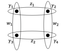
If we consider 4 localised Majorana fermions as shown in the figure below, we can write their Hilbert space by grouping them as shown in the figure. Consider $z_i$ and $w_i$ fermionic modes resulting from the Majorana fermions $\gamma$ :

$z_1=(\gamma_{1}+i\gamma_2)/2, \,\, z_2=(\gamma_{3}+i\gamma_4)/2, \,\, w_1=(\gamma_{1}+i\gamma_3)/2, \,\,\, w_2=(\gamma_{2}+i\gamma_4)/2$

Figure 1: Figure showing four localised Majorana fermions $\gamma_1,\gamma_2,\gamma_3$ and $\gamma_4$ , paired together to give fermionic modes $z_1,z_2$ and $w_1,w_2$ .

These fermionic modes have the vacuum as their total fusion channel and obey the following anticommutation relations:

$\{z_i,z_i^{\dagger}\}=1,{} \{w_i,w_i^{\dagger}\}=1$

Moreover, the operators $z_i^{\dagger}z_i$ and $w_i^{\dagger}w_i$ act on the states that correspond to populated modes, whereas operators $z_iz_i^{\dagger}$ and $w_iw_i^{\dagger}$ act on the zero-population states:

$z_1^{\dagger}z_1\left|00\right>_z=0 , \,\,\,\, z_1^{\dagger}z_1\left|11\right>_z=\left|11\right>_z , \,\,\,\, z_1z_1^{\dagger}\left|00\right>_z=\left|00\right>_z , \,\,\,\, z_1z_1^{\dagger}\left|11\right>_z=0$

Then, based on the aforementioned properties of Majorana fermions and with the help of the creation and annihilation operators we were able to derive the corresponding fusion matrix, $F_M$ for the Majorana fermions given below:

$F_{M}= \frac{1}{\sqrt{2}} \begin{pmatrix} 1 & -1 \\ 1 & 1 \end{pmatrix}$

Notice that, this is the same as the F fusion matrix from the Ising anyon model that we have derived before. We can check that by changing the basis for the $z$ fermions while keeping the same basis for the $w$ ones. We are able to do such a change of basis since the transformation is between two different systems.

Then, considering the braiding properties of the Majorana fermions and choosing to exchange two of them, we were able to derive the corresponding matrices describing their braiding evolution. Again using the creation and annihilation operators, we ended up with the following two matrices, $U$ and $\tilde{U}$ :

$U= e^{i\frac{\pi}{4}} \begin{pmatrix} 0 & 1 \\ 1 & 0 \end{pmatrix}$

$\tilde{U}= e^{-i\frac{\pi}{4}} \begin{pmatrix} 0 & 1 \\ 1 & 0 \end{pmatrix}$

Notice that these are the same as the braiding matrices, $B$ and $\tilde{B}$ , for the Ising anyons.

Discussion of the Results

The Pentagon and Hexagon identities were used to evaluate the fusion and braiding matrices for the Ising anyons. These identities are used in Quantum Field Theory and Topological Field Theory, however they are very abstract. For that, we then made use of the creation and annihilation operators for the Majorana fermions only to end up with the same fusion and braiding matrices as the ones for Ising anyons. Hence, we are able to conclude that indeed “Ising anyons describe the statistical properties of Majorana fermions”.
A more detailed analysis of the results is provided below:

For the case of Ising anyons:

The fusion matrix for the Ising anyons, $F^{\sigma}_{\sigma\sigma\sigma}$ , describes the rearrangement of fusion order between three $\sigma$ anyons, with total fusion outcome $\sigma$ .
We can explain $R_{\sigma\sigma}$ , $\tilde{R}_{\sigma\sigma}$ , $B$ and $\tilde{B}$ by the following statement. If one traverses the braiding in the opposite way, then it is the same as taking the hermitian conjugate of the initial evolution. Indeed, we can see that the two expressions of $B$ and $\tilde{B}$ , are related by a hermitian conjugation $B^{\dagger}=\tilde{B}$ . Note that it is our choice of how we will define our positive, and consequently negative, direction for the braiding.

For the case of Majorana fermions:

The fusion matrix in this case, $F_M$ , describes the fusion between two fermionic modes with their total fusion outcome being the vacuum.
Then, the two different evolutions $U$ and $\tilde{U}$ describe the braiding of two Majorana fermions belonging to two different fermionic modes. Note that the choice between a clockwise and counterclockwise braiding of the two Majorana fermions, results into the two different braiding evolutions $U$ and $\tilde{U}$ .
In general, for an evolution operator $U$ given by $U=e^{-iHt}$ , with $H$ being a hermitian hamiltonian, if we set $t$ to $-t$ we can notice that our evolution operator becomes $U^{\dagger}$ . Thus, it coincides with what we have derived for the evolutions $B$ and $\tilde{B}$ , as well as $U$ and $\tilde{U}$ .