The Ising Model

A useful example is the application of $D_{\mathcal{F}}$ to the 1D ferromagnetic/antiferromagnetic Ising model in both transverse and longitudinal fields, which we discuss here. It is a good idea to first understand the 1D ferromagnetic Ising model and the interactions that take place between the spins. The Hamiltonian for the Ising model is defined as:

$\displaystyle \hat{H} = -\sum_{j=1}^{L}\left(\pm\sigma_{j}^{x}\sigma_{j+1}^{x} + h_{z}\sigma_{j}^{z} + h_{x}\sigma_{j}^{x}\right)$

where $h_{x}$ is the longitudinal field and $h_{z}$ is the transverse field, and $\sigma_{j}^{x, y, z}$ are the Pauli spin matrices acting on site $j$ . By initially taking $h_{x} = 0$ and the first term as positive, we can first consider the ferromagnetic transverse Ising model:

$\displaystyle \hat{H} = -\sum_{j=1}^{L}\sigma_{j}^{x}\sigma_{j+1}^{x} + h_{z}\sum_{j=1}^{L}\sigma_{j}^{z}$

It is well-known that this Hamiltonian is non-interacting because it can be transformed into a free fermion model by performing the Jordan-Wigner transformation. This yields a model with free fermions and the ground state energy

$\displaystyle E_{\pm} = \pm\sqrt{1 + h_{z}^{2} - 2h_{z}cos(k)},$

despite the fact the original spin model naively appeared to be interacting. Thus, the Ising model is a good benchmark for the calculation of interaction distance in the spin model, as we know we should be getting the result $D_\mathcal{F}=0$ .

NB: Another, more intuitive, way of determining if the system is free is to look at a plot of the entanglement spectrum (such as this free, random spectrum):

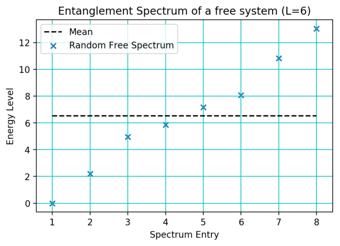
In a free system, the discrete energy levels are constructed as all possible sums of the single particle energies:

$\xi_{a} = \sum_{k}n_{k}(a)m_{k} + z$

Where $n_{k}(a)$ is the occupation of site $k$ in the state $a$ , $m_{k}$ is the single body energy at site k and $z$ is overall normalisation which fixes the trace of the reduced density matrix to be 1.

For this reason, it is clear that the energy levels should be symmetric about the mean value of all levels (as plotted above). Interactions introduce deviations from this symmetry.

Computing the Entanglement Spectrum

To confirm the predicted result, we now go through the process of calculating $\mathcal{D}_{\mathcal{F}}$ for the ground state of the initial spin Hamiltonian.

To proceed, we take a system of a certain size and calculate the Hamiltonian matrix for it. For this example, we shall consider a system where $L=6$ . We label the states such that $|1\rangle$ represents spin-up and $|0\rangle$ represents spin-down. Then for a system containing 6 spins, the basis states are denoted such as $|000001\rangle$ , where this state represents all sites in spin-down, except for the last which is spin-up.
We then act the Hamiltonian according to its original spin form on all possible $\left(2^{L} = 64\right)$ states in order to construct a $2^{L}$ x $2^{L}$ matrix containing the prefactors determined by the Hamiltonian:

$\displaystyle \begin{bmatrix}-6 & 0 & 0 & -1 & \cdots & 0 \\ 0 & \ddots & & & & \\ 0 & & \ddots & & & \\ -1 & & & \ddots & & \\ \vdots & & & & \ddots & \\ 0 & & & & & 6\end{bmatrix}$

By finding the eigenstates of the Hamiltonian, we can then determine the groundstate as the one with the smallest corresponding energy eigenvalue.

As explained here, an important step in calculating $\mathcal{D}_{\mathcal{F}}$ is taking the partial trace of the groundstate when divided into two subsystems. We use the convention of a symmetric bipartition of the system, in this case splitting it into two subsystems of $n=3$ spins. Taking this partial trace gives us a $2^{n} \times 2^{n}$ matrix, $\rho_{A}$ , the reduced density matrix. It is customary to normalise the reduced density such that its trace $Tr\left(\rho_{A}\right) = 1$ .

The final step before calculating $\mathcal{D}_{\mathcal{F}}$ is to obtain the entanglement spectrum. This is defined as the set of eigenvalues of the reduced density matrix, $\rho_{A}$ . Since $\rho_{A}$ has a trace of 1, it is defined as the probability entanglement spectrum. We can also convert it to an energy entanglement spectrum by taking the negative logarithm of each of the values. This will become important later when we go to calculate $\mathcal{D}_{\mathcal{F}}$ using the esfactor repository.

Calculation of $\mathcal{D}_{\mathcal{F}}$

An example entanglement spectrum for the 1D transverse Ising model is given below, for a system of 6 spins that is bipartitioned with open boundary conditions:

$\displaystyle S = \begin{bmatrix}0.11 & 2.30 & 8.63 & 10.82 & 18.30 & 20.49 & 26.82 & 29.01\end{bmatrix}$

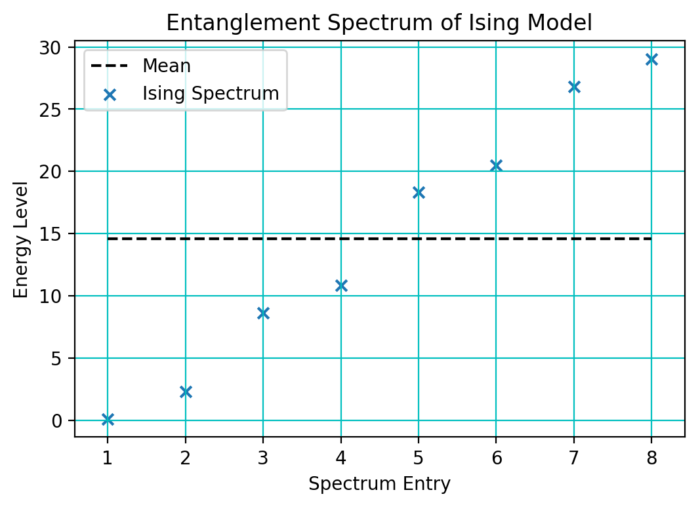
As mentioned previously, it is easy to tell that this spectrum is free by looking at the plot and seeing that the energy levels are symmetric about the mean. We use this entanglement spectrum as the argument to the esfactor.optimise.minimise(...) function, which will calculate $\mathcal{D}_{\mathcal{F}}$ and the single body energies of the system. The results are output as follows:
{ 'N': (100, 23570), 'T': 14.219000101089478, 'ansatz': 'FermionAnsatz', 'converged': True, 'cost': 1.1464786792656745e-16, 'ftol': 1e-06, 'hopping': True, 'm_k': array([ 2.19214288, 8.51959828, 18.19415824]), 'method': 'Nelder-Mead', 'normed': True, 'qm': None, 'qz': None, 'xtol': None, 'z': 0.10606936111744662 }
The important parts of the output are highlighted, namely the cost and m_k. These are the value of $\mathcal{D}_{\mathcal{F}}$ and the single body entanglement energies, respectively. As expected, the value of $\mathcal{D}_{\mathcal{F}}$ is zero within machine precision. Moreover, we can use the single body energies to construct the entanglement spectrum of the closest free system; if this entanglement system is close to that of the Ising entanglement spectrum, it is further proof that the system can be modelled entirely as a free system. This is easily verified:

$\displaystyle \mathrm{Ising} = \begin{bmatrix}0.11&2.30&8.63&10.82&18.30&20.49&26.82&29.01\end{bmatrix} \\ \mathrm{Free Approx.} = \begin{bmatrix}0&2.19&8.52&10.71&18.19&20.39&26.71&28.91\end{bmatrix}$

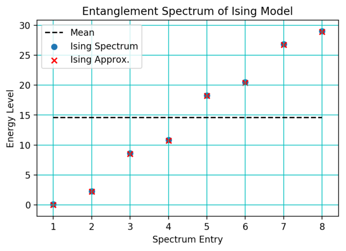
As can be seen, there is excellent agreement between the two spectra, which confirms that the ferromagnetic transverse Ising system can indeed be modelled by free fermions.

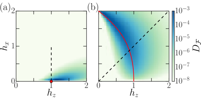
For each pixel of these graphs esfactor was used to calculate [latex]D_\mathcal{F}[/latex]

Now that we have demonstrated that $D_{\mathcal{F}}$ is able to identify a free state even in the "wrong" basis, we can map out the phase diagram as a function of two parameters of the Ising model, the longitudinal and transverse fields, $h_x$ and $h_z$ .

In the above figure (taken from the first paper), figure (a) is the phase diagram for the ferromagnetic Ising model, while (b) shows the same for the antiferromagnetic Ising model. In (a), the point $(h_z = 1, h_x = 0)$ is what was calculated in the above example. As expected, the colour map shows the entire line $h_x = 0$ is completely free with $D_{\mathcal{F}} = 0$ . A surprising aspect of this phase diagram is that, apart from the close vicinity of the critical point or critical line (red dot and red line), the system is nearly free otherwise, as evidenced by the light coloured areas in the phase diagram. We have also computed the optimal free model throughout the phase diagram, as explained here.