Mapping to Free Fermions

The Jordan-Wigner transformation is used to transform a Hamiltonian from an interacting spin basis (such as the standard transverse Ising Hamiltonian shown below) into a non-interacting fermionic basis. As it is well known, we start from the Hamiltonian

$\displaystyle \hat{H} = -\sum_{j=1}^{L}\sigma_{j}^{x}\sigma_{j+1}^{x} + h_{z}\sum_{j}^{L}\sigma_{j}^{z}$

and then define a new set of fermionic operators from the Pauli operators:

$c_{j}^{\dagger} = e^{+i\pi\sum_{k=1}^{j-1}\sigma_{k}^{+}\sigma_{k}^{-}} \cdot \sigma_{j}^{+} \newline c_{j} = e^{-i\pi\sum_{k=1}^{j-1}\sigma_{k}^{+}\sigma_{k}^{-}} \cdot \sigma_{j}^{-} \newline c_{j}^{\dagger}c_{j} = \sigma_{j}^{+}\sigma_{j}^{-} \newline \sigma_{j}^{z} = 2\sigma_{j}^{+}\sigma_{j}^{-} - 1 = 2c_{j}^{\dagger}c_{j} - 1$

The exponentials in $c_{j}^{\dagger}$ and $c_{j}$ are more commonly expressed as:

$\displaystyle e^{\pm\sum_{k=1}^{j-1}\sigma_{k}^{+}\sigma_{k}^{-}} = \prod_{k=1}^{j-1}e^{\pm\sigma_{k}^{+}\sigma_{k}^{-}} = \prod_{k=1}^{j-1}\left(1-2\sigma_{k}^{+}\sigma_{k}^{-}\right) = \prod_{k=1}^{j-1}\left(1-2n_{k}\right)$

where we have defined a new operator, $n_{k}\equiv c_k^\dagger c_k$ . This is the occupation operator and returns a 1 if the site $k$ is occupied and a 0 if not. We can then re-write $\hat{H}$ in terms of these new fermionic operators, by taking the previous result for $\sigma_{j}^{z}$ and the equality:

$\displaystyle \sigma_{j}^{x} = \frac{\sigma_{j}^{+} + \sigma_{j}^{-}}{2} = \prod_{k=1}^{j-1}\left( 1 - 2n_{k}\right)\left(c_{j} + c_{j}^{\dagger}\right)$

$\displaystyle \rightarrow \sigma_{j}^{x}\sigma_{j+1}^{x} = \prod_{k=1}^{j-1}\left(1-2n_{k}\right)\left(c_{j} + c_{j}^{\dagger}\right) \prod_{k'=1}^{j}\left(1 - 2n_{k'}\right)\left(c_{j+1} + c_{j+1}^{\dagger}\right)$

$\displaystyle \rightarrow \hat{H} = -\sum_{j} \prod_{k=1}^{j-1}\left(1-2n_{k}\right)\left(c_{j} + c_{j}^{\dagger}\right) \prod_{k'=1}^{j}\left(1 - 2n_{k'}\right)\left(c_{j+1} + c_{j+1}^{\dagger}\right) + h_{z}\sum_{j}\sigma_{j}^{z}$

$\displaystyle = -\sum_{i}\left[\prod_{j<i}\left(1 - 2n_{j}\right)\right]^{2} \left(c_{i}^{\dagger} + c_{i}\right)\left(1-2n_{j}\right)\left(c_{i+1}^{\dagger} + c_{i+1}\right)$

From the above equation, it is simple to see that the squared product is always equal to 1, whilst the second and third terms can be expanded to equal $c_{j}^{\dagger} - c_{j}$ . All this combined gives the Hamiltonian in terms of the fermions operators as:

$\displaystyle \hat{H} = -\sum_{j}\left(c_{j}^{\dagger}-c_{j}\right)\left(c_{j+1}+c_{j+1}^{\dagger}\right) + 2h_{z}\sum_{i}c_{i}^{\dagger}c_{i} + const.$

We then take the Fourier Transform of this form of the Hamiltonian to exploit the translation invariance of the system. Let:

$c_{j} = \frac{1}{\sqrt{N}}\sum_{k}e^{ikj}c_{k} \newline c_{j}^{\dagger} = \frac{1}{\sqrt{N}}\sum_{k}e^{-ikj}c_{k}^{\dagger}$

Then:

$\displaystyle \hat{H} = -\sum_{j}\left(c_{j}^{\dagger}c_{j+1} + c_{j+1}^{\dagger}c_{j}\right) - \sum_{j}\left(c_{j}^{\dagger}c_{j+1}^{\dagger} + c_{j+1}c_{j}\right) + 2h_{z}\sum_{j}n_{j} \newline = -\sum_{k}c_{k}^{\dagger}c_{k}\left[2cos(k)\right] - \sum_{k}\left(c_{k}^{\dagger}c_{-k}^{\dagger}e^{ik} + c_{-k}c_{k}e^{-ik}\right) + 2h_{z}\sum_{k}c_{k}^{\dagger}c_{k}$

We want to rewrite this as:

$\displaystyle \sum_{k}\begin{pmatrix}c_{k}^{\dagger}& c_{-k}\end{pmatrix}\begin{pmatrix} H_{11}(k)&H_{12}(k)\\H_{21}(k)&H_{22}(k) \end{pmatrix}\begin{pmatrix}c_{k}\\c_{-k}^{\dagger}\end{pmatrix}$

and this can be acheived by splitting each of the previous terms into 2 sums of half the original value, it can be shown that we arrive at:

$\displaystyle \hat{H} = \sum_{k}\left(c_{k}^{\dagger}c_{k} + c_{-k}^{\dagger}c_{-k}\right)\left(-cos(k) + h_{z}\right) + \sum_{k}\left(-isin(k) c_{k}^{\dagger}c_{-k}^{\dagger} + isin(k)c_{-k}c_{k}\right)$

$\displaystyle = \sum_{k}\begin{pmatrix}c_{k}^{\dagger}&c_{-k}\end{pmatrix}\begin{pmatrix}-cos(k)+h_{z}&-isin(k)\\isin(k)&cos(k)-h_{z}\end{pmatrix}\begin{pmatrix}c_{k}\\c_{-k}^{\dagger}\end{pmatrix}$

By diagonalising the kernel matrix, we can then find the eigenvalues of the Hamiltonian. It is simple to see that it gives two energy bands:

$E_{\pm} = \pm\sqrt{1+h_{z}^{2}-2h_{z}cos(k)},$

where $k=2\pi \tilde{k}/L$ , $\tilde k = 0, 1, \ldots, L-1$ . Since the Hamiltonian is diagonalisable, it shows that the initial 1D Ising model of spins can be completely described by free fermions filling the energy levels above.

The natural question is whether a free model exists once the Ising model is perturbed by longitudinal field, which in the Jordan-Wigner picture introduces interactions between fermions. Since we have previously established that $D_\mathcal{F}$ is small in large parts of the phase diagram, even where longitudinal field $h_x$ is strong, we expect such a free model should exist. It turns out that the optimal free model is the free Ising model, as illustrated in figure below.

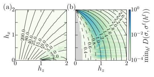
The above figure is a sophisticated way of visualising the success of using interaction distance to map the optimal free model of an interacting ground state to a system of free fermions, namely the transverse Ising model ( $h_x = 0$ ). The isobars show what value of transverse field $h_z$ one would need in the free model in order to have a ground state close to the interacting model at that given point. The colour map shows the success of this mapping, measured by the value of $D_\mathcal{F}$ . Similar identification of a free model can be performed in the antiferromagnetic case (b).